Tutorial: TraceFitter
In following documentation we will explain how to get started with using
TraceFitter. Here we will optimize conductances for
a Hodgkin-Huxley cell model.
We start by importing brian2 and brian2modelfitting:
from brian2 import *
from brian2modelfitting import *
Problem description
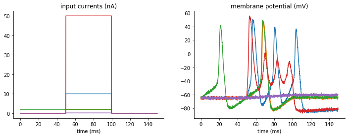
We have five step input currents of different amplitude and five “data samples”
recorded from the model with goal parameters. The goal of this exercise is to
optimize the conductances of the model gl, g_na, g_kd, for which we
know the expected ranges.
Visualization of input currents and corresponding output traces which we will try to fit:
We can load these currents and “recorded” membrane potentials with the pandas library
import pandas as pd
inp_trace = pd.read_csv('input_traces_hh.csv', index_col=0).to_numpy()
out_trace = pd.read_csv('output_traces_hh.csv', index_col=0).to_numpy()
Note
You can download the CSV files used above here:
input_traces_hh.csv,
output_traces_hh.csv
Procedure
Model definition
We have to specify all of the constants for the model
area = 20000*umetre**2
Cm=1*ufarad*cm**-2 * area
El=-65*mV
EK=-90*mV
ENa=50*mV
VT=-63*mV
Then, we have to define our model:
model = '''
dv/dt = (gl*(El-v) - g_na*(m*m*m)*h*(v-ENa) - g_kd*(n*n*n*n)*(v-EK) + I)/Cm : volt
dm/dt = 0.32*(mV**-1)*(13.*mV-v+VT)/
  (exp((13.*mV-v+VT)/(4.*mV))-1.)/ms*(1-m)-0.28*(mV**-1)*(v-VT-40.*mV)/
  (exp((v-VT-40.*mV)/(5.*mV))-1.)/ms*m : 1
dn/dt = 0.032*(mV**-1)*(15.*mV-v+VT)/
  (exp((15.*mV-v+VT)/(5.*mV))-1.)/ms*(1.-n)-.5*exp((10.*mV-v+VT)/(40.*mV))/ms*n : 1
dh/dt = 0.128*exp((17.*mV-v+VT)/(18.*mV))/ms*(1.-h)-4./(1+exp((40.*mV-v+VT)/(5.*mV)))/ms*h : 1
g_na : siemens (constant)
g_kd : siemens (constant)
gl   : siemens (constant)
'''
Note
You have to identify the parameters you want to optimize by adding them as constant variables to the equation.
Optimizer and metric
Once we know our model and parameters, it’s time to pick an optimizing algorithm and a metric that will be used as a measure.
For simplicity we will use the default method provided by the
NevergradOptimizer, i.e.
“Differential Evolution”, and the MSEMetric,
calculating the mean squared error between simulated and data traces:
opt = NevergradOptimizer()
metric = MSEMetric()
Fitter Initiation
Since we are going to optimize over traces produced by the model, we need to
initiate the fitter TraceFitter:
The minimum set of input parameters for the fitter, includes the model
definition, input and output variable names and traces,
time step dt, number of samples we want to draw in each optimization round.
fitter = TraceFitter(model=model,
                     input={'I': inp_trace*amp},
                     output={'v': out_trace*mV},
                     dt=0.01*ms, n_samples=100, method='exponential_euler',
                     param_init={'v': -65*mV})
Additionally, in this example, we pick the integration method to be
'exponential_euler', and we specify the initial value of the state variable
v, by using the option: param_init={'v': -65*mV}.
Fit
We are now ready to perform the optimization, by calling the
fit method. We need to pass the
optimizer, metric and pick a number of rounds(n_rounds).
Note
Here you have to also pass the ranges for each of the parameters that was defined as a constant!
res, error = fitter.fit(n_rounds=10,
                        optimizer=opt,
                        metric=metric,
                        gl=[2*psiemens, 200*nsiemens],
                        g_na=[200*nsiemens, 0.4*msiemens],
                        g_kd=[200*nsiemens, 200*usiemens])
- Output:
res: dictionary with best fit values from this optimizationerror: corresponding error
The default output during the optimization run will tell us the best parameters in each round of optimization and the corresponding error:
Round 0: fit [9.850944960633812e-05, 5.136956717618642e-05, 1.132001753695881e-07] with error: 0.00023112503428419085
Round 1: fit [2.5885625978001192e-05, 5.994175009416155e-05, 1.132001753695881e-07] with error: 0.0001351283127819249
Round 2: fit [2.358033085911261e-05, 5.2863196016834924e-05, 7.255743458079185e-08] with error: 8.600916130059129e-05
Round 3: fit [2.013515980650059e-05, 4.5888592959196316e-05, 7.3254174819061e-08] with error: 5.704891495098806e-05
Round 4: fit [9.666300621928093e-06, 3.471303670631636e-05, 2.6927249265934296e-08] with error: 3.237910401003197e-05
Round 5: fit [8.037164838105382e-06, 2.155149445338687e-05, 1.9305129338706338e-08] with error: 1.080794896277778e-05
Round 6: fit [7.161113899555702e-06, 2.2680883630214104e-05, 2.369859751788268e-08] with error: 4.527456021770018e-06
Round 7: fit [7.471475084450997e-06, 2.3920164839406964e-05, 1.7956856689140395e-08] with error: 4.4765688852930405e-06
Round 8: fit [6.511156620775884e-06, 2.209792671051356e-05, 1.368667359118384e-08] with error: 1.8105782339584402e-06
Round 9: fit [6.511156620775884e-06, 2.209792671051356e-05, 1.368667359118384e-08] with error: 1.8105782339584402e-06
Generating traces
To generate the traces that correspond to the new best fit parameters of the
model, you can use the generate_traces
method.
traces = fitter.generate_traces()
The following plot shows the fit traces in comparison to our target data:
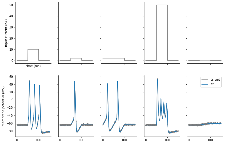
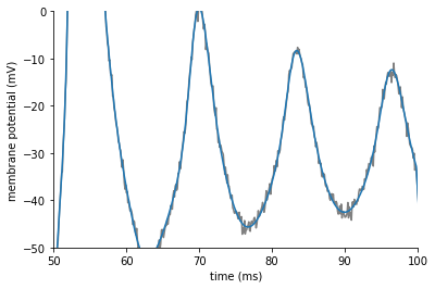
The fit looks good in general, but if we zoom in on the fourth column we see that the fit is still not perfect:
We can improve the fit by using a classic, sequential curve fitting algorithm.
Refining fits
When using TraceFitter, you can further refine the fit by
applying a standard least squares fitting algorithm (e.g. Levenberg–Marquardt), by calling
refine. By default, this will start from the
previously found best parameters:
refined_params, result_info = fitter.refine()
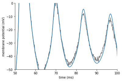
We can now generate traces with the refined parameters:
traces = fitter.generate_traces(params=refined_params)
Plotting the results, we see that the fits have improved and now closely match the target data: