Tutorial: Inferencer
In this tutorial, we use simulation-based inference on the Hodgkin-Huxley neuron model, [Hodgkin1952], where different scenarios are considered. The data are synthetically generated from the model which enables the comparisson of the optimized parameter values with the ground truth parameter values as used in the generative model.
We start with importing basic packages and modules. Note that
tutorial_sbi_helpers contains three different functions that are used
extensively throughout this tutorial. Namely, plot_traces is used for
visualization of the input current and output voltage traces, and optionally
for visualization of spike trains or sampled traces obtained by using an
estimated posterior. In order to detect and capture spike events in a given
voltage trace, we use spike_times function. Finally,
plot_cond_coeff_mat is used to visualize conditional coerrelation matrix.
For a detailed overview of the mechanism of each of the functions, download
the script: tutorial_sbi_helpers.py
from brian2 import *
from brian2modelfitting import Inferencer
from scipy.stats import kurtosis as kurt
from tutorial_sbi_helpers import (spike_times,
                                  plot_traces,
                                  plot_cond_coeff_mat)
Now, let’s load the input current and output voltage traces by using NumPy.
Note that all functions available in NumPy, as well as in Matplotlib,
are implicitly available after brian2 was imported.
inp_traces = load('input_traces_synthetic.npy').reshape(1, -1)
out_traces = load('output_traces_synthetic.npy').reshape(1, -1)
The data is generated by running generate_traces_synthetic.py script:
generate_traces_synthetic.py
By setting the time step, we are able to set up the time domain. From the
array of time steps, we also define the exact time when the stimulus starts
and when it ends by computing stim_start and stim_end, respectively.
This will come handy later during the feature extraction process.
dt = 0.05*ms
t = arange(0, inp_traces.size*dt/ms, dt/ms)
stim_start, stim_end = t[where(inp_traces[0, :] != 0)[0][[0, -1]]]
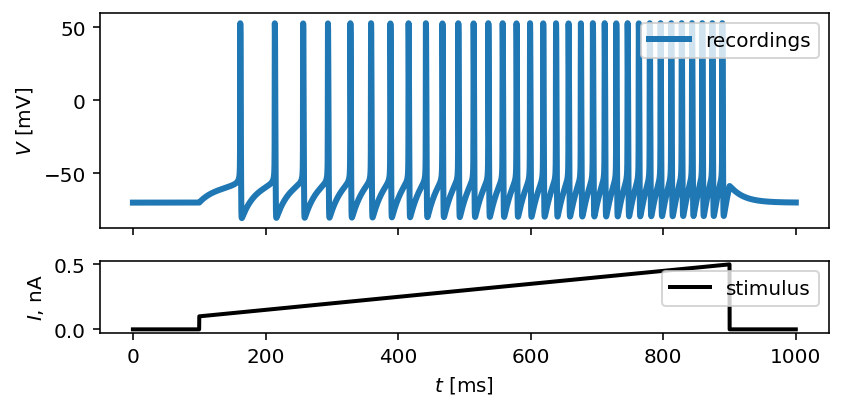
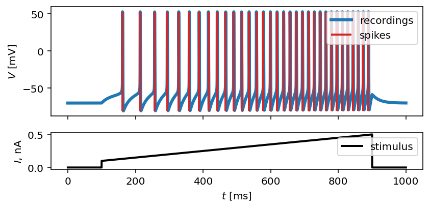
By calling plot_traces and passing the array of time steps, the input
current and output voltage traces, we obtain the visualization of a synthetic
neural activity recordings:
fig, ax = plot_traces(t, inp_traces, out_traces)
Toy-example: infer two free parameters
The first scenario we cover is a simple inference procedure of two unknown parameters in the Hodgkin-Huxley neuron model. The parameters to infer are the maximal value of sodium, \(\overline{g}_\mathrm{Na}\), and potassium electrical conductances, \(\overline{g}_\mathrm{K}\).
By following the standard practice from Brian 2 simulator, we have to define parameters of the model, initial conditions for differential equations that describe the model, and the model itself:
# set parameters of the model
E_Na = 53*mV
E_K = -107*mV
E_l = -70*mV
VT = -60.0*mV
g_l = 10*nS
Cm = 200*pF

# set ground truth parameters, which are unknown from the model's perspective
ground_truth_params = {'g_Na': 32*uS,
                       'g_K': 1*uS}

# define initial conditions
init_conds = {'v': 'E_l',
              'm': '1 / (1 + beta_m / alpha_m)',
              'h': '1 / (1 + beta_h / alpha_h)',
              'n': '1 / (1 + beta_n / alpha_n)'}

# define the Hodgkin-Huxley neuron model
eqs = '''
    # non-linear set of ordinary differential equations
    dv/dt = - (g_Na * m ** 3 * h * (v - E_Na)
               + g_K * n ** 4 * (v - E_K)
               + g_l * (v - E_l) - I) / Cm : volt
    dm/dt = alpha_m * (1 - m) - beta_m * m : 1
    dn/dt = alpha_n * (1 - n) - beta_n * n : 1
    dh/dt = alpha_h * (1 - h) - beta_h * h : 1

    # time independent rate constants for a channel activation/inactivation
    alpha_m = ((-0.32 / mV) * (v - VT - 13.*mV))
               / (exp((-(v - VT - 13.*mV)) / (4.*mV)) - 1) / ms : Hz
    beta_m = ((0.28/mV) * (v - VT - 40.*mV))
              / (exp((v - VT - 40.*mV) / (5.*mV)) - 1) / ms : Hz
    alpha_h = 0.128 * exp(-(v - VT - 17.*mV) / (18.*mV)) / ms : Hz
    beta_h = 4 / (1 + exp((-(v - VT - 40.*mV)) / (5.*mV))) / ms : Hz
    alpha_n = ((-0.032/mV) * (v - VT - 15.*mV))
               / (exp((-(v - VT - 15.*mV)) / (5.*mV)) - 1) / ms : Hz
    beta_n = 0.5 * exp(-(v - VT - 10.*mV) / (40.*mV)) / ms : Hz

    # free parameters
    g_Na : siemens (constant)
    g_K : siemens (constant)
    '''
Since the output of the model is extremely high-dimensional, and since we are interested only in a few hand-picked features that will capture the gist of the neuronal activity, we start the inference process by defining a list of summary functions.
Each summary feature is obtained by calling a single-valued function on each trace generated by using a sampled prior distribution over unknown parameters. In this case, we consider the maximal value, mean and standard deviatian of action potential, and the membrane resting potential.
v_features = [
    # max action potential
    lambda x: np.max(x[(t > stim_start) & (t < stim_end)]),
    # mean action potential
    lambda x: np.mean(x[(t > stim_start) & (t < stim_end)]),
    # std of action potential
    lambda x: np.std(x[(t > stim_start) & (t < stim_end)]),
    # membrane resting potential
    lambda x: np.mean(x[(t > 0.1 * stim_start) & (t < 0.9 * stim_start)])
]
Inferencer
The minimum set of arguments for the Inferencer
class constructor are the time step, dt, input data traces, input,
output data traces, output, and the model that will be used for the
inference process, model. Input and output traces should have the number
of rows that corresponds to the number of observed traces, and the number of
columns should be equal to the number of time steps in each trace.
Here, we define additional arguments such as: method to define an
integration technique used for solving the set of differential equations,
threshold to define a condition that produce a single spike, refractory
to define a condition under which a neuron remains refractory, and
param_init to define a set of initial conditions. We also define the set of
summary features that is used to represent the data instead of using the entire
trace. Summary features are passed to the inference algorithm via features
argument.
inferencer = Inferencer(dt=dt, model=eqs,
                        input={'I': inp_traces*amp},
                        output={'v': out_traces*mV},
                        features={'v': v_features},
                        method='exponential_euler',
                        threshold='m > 0.5',
                        refractory='m > 0.5',
                        param_init=init_conds)
After the inferencer is instantiated, we may begin the inference process
by calling infer and defining the
total number of samples that are used for the training of a neural density
estimator. We use the sequential neural posterior estimation algorithm (SNPE),
proposed in [Greenberg2019].
Posterior
Neural density estimator learns the probabilistic mapping of the input data, i.e., sampled parameter values given a prior distribution, and the output data, i.e., summary features extracted from the traces, obtained by solving the model with the corresponding set of sampled parameters from the input data.
We can choose the inference method and the estimator model , but only
arguments that infer requires are
the number of samples (in case of running the inference process for the first
time), n_samples, and upper and lower bounds for each unknown parameter.
posterior = inferencer.infer(n_samples=15_000,
                             n_rounds=1,
                             inference_method='SNPE',
                             density_estimator_model='maf',
                             g_Na=[1*uS, 100*uS],
                             g_K=[0.1*uS, 10*uS])
After inference is completed, the estimated posterior distribution can be analyzed by observing the pairwise relationship between each pair of parameters. But before, we have to draw samples from the estimated posterior as follows:
samples = inferencer.sample((10_000, ))
The samples are stored inside the Inferencer
object and are available through samples variable.
We create a visual representation of the pairwise relationship of the posterior
as follows:
limits = {'g_Na': [1*uS, 100*uS],
          'g_K': [0.1*uS, 10*uS]}
labels = {'g_Na': r'$\overline{g}_{Na}$',
          'g_K': r'$\overline{g}_{K}$'}
fig, ax = inferencer.pairplot(limits=limits,
                              labels=labels,
                              ticks=limits,
                              points=ground_truth_params,
                              points_offdiag={'markersize': 5},
                              points_colors=['C3'],
                              figsize=(6, 6))
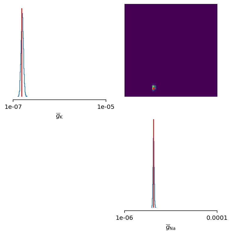
Let’s zoom in a bit:
The inferred posterior is plotted against the ground truth parameters, and as can be seen, the ground truth parameters are located in high-probability regions of the estimated distribution.
To further substantiate this, let’s now see the traces simulated from a single set of parameters sampled from the posterior:
inf_traces = inferencer.generate_traces()
We again use the plot_traces function as follows:
fig, ax = plot_traces(t, inp_traces, out_traces, inf_traces=array(inf_traces/mV))
Additional free parameters
The simple scenarios where only 2 parameters are considered works quite well using synthetic data traces. What if we have a larger number of unkown parameters? Let’s now consider additional unkown parameters for the same model as before. In addition to the unknown maximal values of the electrical conductance of the sodium and potassium channels, the membrane capacity, \(C_m\), and the maximal value of the electrical conductance of the leakage ion channel, \(\overline{g}_{l}\), are also unknown.
We can try to do the same as before with a bit more training data:
del Cm, g_l
# set parameters, initial condition and the model
E_Na = 53*mV
E_K = -107*mV
E_l = -70*mV
VT = -60.0*mV
ground_truth_params = {'g_Na': 32*uS,
'g_K': 1*uS,
'g_l': 10*nS,
'Cm': 200*pF}
init_conds = {'v': 'E_l',
'm': '1 / (1 + beta_m / alpha_m)',
'h': '1 / (1 + beta_h / alpha_h)',
'n': '1 / (1 + beta_n / alpha_n)'}
eqs = '''
# non-linear set of ordinary differential equations
dv/dt = - (g_Na * m ** 3 * h * (v - E_Na)
+ g_K * n ** 4 * (v - E_K)
+ g_l * (v - E_l) - I) / Cm : volt
dm/dt = alpha_m * (1 - m) - beta_m * m : 1
dn/dt = alpha_n * (1 - n) - beta_n * n : 1
dh/dt = alpha_h * (1 - h) - beta_h * h : 1
# time independent rate constants for activation and inactivation
alpha_m = ((-0.32 / mV) * (v - VT - 13.*mV))
/ (exp((-(v - VT - 13.*mV)) / (4.*mV)) - 1) / ms : Hz
beta_m = ((0.28/mV) * (v - VT - 40.*mV))
/ (exp((v - VT - 40.*mV) / (5.*mV)) - 1) / ms : Hz
alpha_h = 0.128 * exp(-(v - VT - 17.*mV) / (18.*mV)) / ms : Hz
beta_h = 4 / (1 + exp((-(v - VT - 40.*mV)) / (5.*mV))) / ms : Hz
alpha_n = ((-0.032/mV) * (v - VT - 15.*mV))
/ (exp((-(v - VT - 15.*mV)) / (5.*mV)) - 1) / ms : Hz
beta_n = 0.5 * exp(-(v - VT - 10.*mV) / (40.*mV)) / ms : Hz
# free parameters
g_Na : siemens (constant)
g_K : siemens (constant)
g_l : siemens (constant)
Cm : farad (constant)
'''
# infer the posterior using the same configuration as before
inferencer = Inferencer(dt=dt, model=eqs,
input={'I': inp_traces*amp},
output={'v': out_traces*mV},
features={'v': v_features},
method='exponential_euler',
threshold='m > 0.5',
refractory='m > 0.5',
param_init=init_conds)
posterior = inferencer.infer(n_samples=20_000,
n_rounds=1,
inference_method='SNPE',
density_estimator_model='maf',
g_Na=[1*uS, 100*uS],
g_K=[0.1*uS, 10*uS],
g_l=[1*nS, 100*nS],
Cm=[20*pF, 2*nF])
# finally, sample and visualize the posterior distribution
samples = inferencer.sample((10_000, ))
limits = {'g_Na': [1*uS, 100*uS],
'g_K': [0.1*uS, 10*uS],
'g_l': [1*nS, 100*nS],
'Cm': [20*pF, 2*nF]}
labels = {'g_Na': r'$\overline{g}_{Na}$',
'g_K': r'$\overline{g}_{K}$',
'g_l': r'$\overline{g}_{l}$',
'Cm': r'$C_{m}$'}
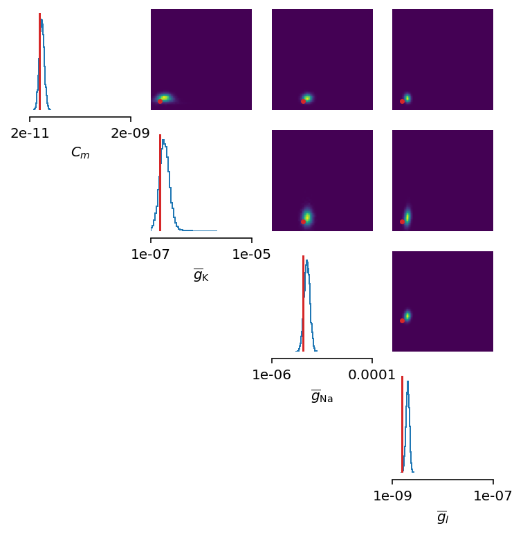
fig, ax = inferencer.pairplot(limits=limits,
labels=labels,
ticks=limits,
points=ground_truth_params,
points_offdiag={'markersize': 5},
points_colors=['C3'],
figsize=(6, 6))
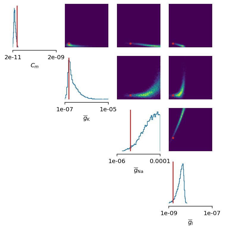
This could have been expected. The posterior distribution is estimated poorly using a simple approach as in the toy example.
Yes, we can play around with hyper-parameters and tuning the neural density estimator, but with this apporach we will not get far.
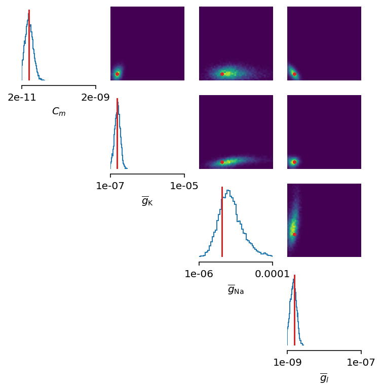
We can, however, try with the non-amortized (or focused) approach, meaning we perform multi-round inference, where each following round will use the posterior from the previous one to sample new input data for the training, rather than using the same prior distribution as defined in the beginning. This approach yields additional advantage - the number of samples may be considerably lower, but it will lead to the posterior that is no longer being amortized - it is accurate only for a specific observation.
# note that the only difference is the number of rounds of inference
posterior = inferencer.infer(n_samples=10_000,
                             n_rounds=2,
                             inference_method='SNPE',
                             density_estimator_model='maf',
                             restart=True,
                             g_Na=[1*uS, 100*uS],
                             g_K=[0.1*uS, 10*uS],
                             g_l=[1*nS, 100*nS],
                             Cm=[20*pF, 2*nF])

samples = inferencer.sample((10_000, ))

fig, ax = inferencer.pairplot(limits=limits,
                              labels=labels,
                              ticks=limits,
                              points=ground_truth_params,
                              points_offdiag={'markersize': 5},
                              points_colors=['C3'],
                              figsize=(6, 6))
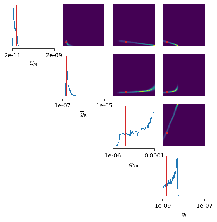
This seems as a promising approach for parameters that already have the high-probability regions of the posterior distribution around ground-truth values. For other parameters, this leads to further deterioration of posterior estimates.
So, we may wonder, how else can we improve the neural density estimator accuracy?
Currently, we use only four features to describe extremely complex output of a neural model and should probably create a more comprehensive and more descriptive set of summary features. If we want to include data related to spikes in summary statistics, it is necessary to perform multi-objective optimization since we will observe spike trains as an output in addition to voltage traces.
Multi-objective optimization
In order to use spikes, we have to have some observation to pass to the
Inferencer. We can utilize spike_times as
follows:
spike_times_list = [spike_times(t, out_trace) for out_trace in out_traces]
To visually prove that spike times are indeed correct, we use plot_traces:
fig, ax = plot_traces(t, inp_traces, out_traces, spike_times_list[0])
Now, let’s create additional features that will be applied to voltage traces, and a few features that will be applied to spike trains:
def voltage_deflection(x):
    voltage_base = np.mean(x[t < stim_start])
    stim_end_idx = np.where(t >= stim_end)[0][0]
    steady_state_voltage_stimend = np.mean(x[stim_end_idx-10:stim_end_idx-5])
    return steady_state_voltage_stimend - voltage_base


v_features = [
    # max action potential
    lambda x: np.max(x[(t > stim_start) & (t < stim_end)]),
    # mean action potential
    lambda x: np.mean(x[(t > stim_start) & (t < stim_end)]),
    # std of action potential
    lambda x: np.std(x[(t > stim_start) & (t < stim_end)]),
    # kurtosis of action potential
    lambda x: kurt(x[(t > stim_start) & (t < stim_end)], fisher=False),
    # membrane resting potential
    lambda x: np.mean(x[(t > 0.1 * stim_start) & (t < 0.9 * stim_start)]),
    # the voltage deflection between base and steady-state voltage
    voltage_deflection,
]

s_features = [
    # number of spikes in a train
    lambda x: x.size,
    # mean inter-spike interval
    lambda x: 0. if np.diff(x).size == 0 else np.mean(diff(x)),
    # time to first spike
    lambda x: 0. if x.size == 0 else x[0]
]
The rest of the inference process stays pretty much the same as before:
inferencer = Inferencer(dt=dt, model=eqs,
                        input={'I': inp_traces*amp},
                        output={'v': out_traces*mV, 'spikes': spike_times_list},
                        features={'v': v_features, 'spikes': s_features},
                        method='exponential_euler',
                        threshold='m > 0.5',
                        refractory='m > 0.5',
                        param_init=init_conds)

posterior = inferencer.infer(n_samples=20_000,
                             n_rounds=1,
                             inference_method='SNPE',
                             density_estimator_model='maf',
                             g_Na=[1*uS, 100*uS],
                             g_K=[0.1*uS, 10*uS],
                             g_l=[1*nS, 100*nS],
                             Cm=[20*pF, 2*nF])

samples = inferencer.sample((10_000, ))

fig, ax = inferencer.pairplot(limits=limits,
                              labels=labels,
                              ticks=limits,
                              points=ground_truth_params,
                              points_offdiag={'markersize': 5},
                              points_colors=['C3'],
                              figsize=(6, 6))

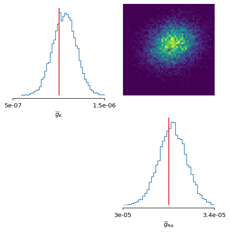
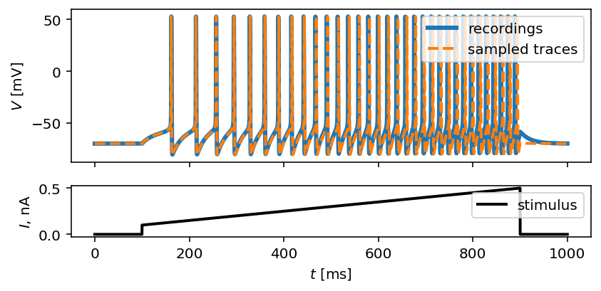
Let’s also visualize the sampled trace, this time using the mean of ten thousands drawn samples:
inf_traces = inferencer.generate_traces(n_samples=10_000, output_var='v')

fig, ax = plot_traces(t, inp_traces, out_traces, inf_traces=array(inf_traces/mV))
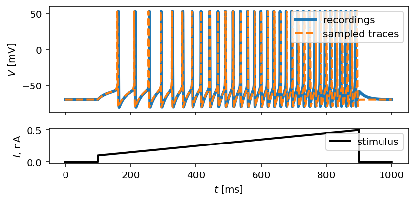
Okay, now we are clearly getting somewhere and this should be a strong indicatior of the importance of crafting quality summary statistics.
Still, the summary statistics can be a huge bottleneck and can set back the training of a neural density estimator. For this reason automatic feature extraction can be considered instead.
Automatic feature extraction
To enable automatic feature extraction, features argument simly should
not be defined when instantiating an inferencer object. And that’s it.
Everything else happens behind the scenes without any need for additional user
intervention. If the user wants to gain additional control over the extraction
process, in addition to changing the hyperparameters, they can also define
their own embedding neural network.
Default settings
inferencer = Inferencer(dt=dt, model=eqs,
                        input={'I': inp_traces*amp},
                        output={'v': out_traces*mV},
                        method='exponential_euler',
                        threshold='m > 0.5',
                        refractory='m > 0.5',
                        param_init=init_conds)

posterior = inferencer.infer(n_samples=20_000,
                             n_rounds=1,
                             inference_method='SNPE',
                             density_estimator_model='maf',
                             g_Na=[1*uS, 100*uS],
                             g_K=[0.1*uS, 10*uS],
                             g_l=[1*nS, 100*nS],
                             Cm=[20*pF, 2*nF])

samples = inferencer.sample((10_000, ))

fig, ax = inferencer.pairplot(limits=limits,
                              labels=labels,
                              ticks=limits,
                              points=ground_truth_params,
                              points_offdiag={'markersize': 5},
                              points_colors=['C3'],
                              figsize=(6, 6))
Custom embedding network
Here, we demonstrate how to build a custom summary feature extractor and how to exploit the GPU processing power to speed up the inference process.
Note that the use of the GPU will result in the speed-up of computation time only if a custom automatic feature extractor uses techniques that are actually faster to compute on the GPU.
For this case, we use the YuleNet, a convolutional neural network, proposed in [Rodrigues2020]. The authors outline impresive results where the automatic feature extraction by using the YuleNet is capable of outperforming carefully hand-crafted features.
import torch
from torch import nn


class YuleNet(nn.Module):
    """The summary feature extractor proposed in Rodrigues 2020.

    Parameters
    ----------
    in_features : int
        Number of input features should correspond to the size of a
        single output voltage trace.
    out_features : int
        Number of the features that are used for the inference process.

    Returns
    -------
    None

    References
    ----------
    * Rodrigues, P. L. C. and Gramfort, A. "Learning summary features
      of time series for likelihood free inference" 3rd Workshop on
      Machine Learning and the Physical Sciences (NeurIPS 2020). 2020.
    """
    def __init__(self, in_features, out_features):
        super().__init__()
        self.conv1 = nn.Conv1d(in_channels=1, out_channels=8, kernel_size=64,
                               stride=1, padding=32, bias=True)
        self.relu1 = nn.ReLU()
        pooling1 = 16
        self.pool1 = nn.AvgPool1d(kernel_size=pooling1)

        self.conv2 = nn.Conv1d(in_channels=8, out_channels=8, kernel_size=64,
                               stride=1, padding=32, bias=True)
        self.relu2 = nn.ReLU()
        pooling2 = int((in_features // pooling1) // 16)
        self.pool2 = nn.AvgPool1d(kernel_size=pooling2)

        self.dropout = nn.Dropout(p=0.50)
        linear_in = 8 * in_features // (pooling1 * pooling2) - 1
        self.linear = nn.Linear(in_features=linear_in,
                                out_features=out_features)
        self.relu3 = nn.ReLU()

    def forward(self, x):
        if x.ndim == 1:
            x = x.view(1, 1, -1)
        else:
            x = x.view(len(x), 1, -1)
        x_conv1 = self.conv1(x)
        x_relu1 = self.relu1(x_conv1)
        x_pool1 = self.pool1(x_relu1)

        x_conv2 = self.conv2(x_pool1)
        x_relu2 = self.relu2(x_conv2)
        x_pool2 = self.pool2(x_relu2)

        x_flatten = x_pool2.view(len(x), 1, -1)
        x_dropout = self.dropout(x_flatten)

        x = self.relu3(self.linear(x_dropout))
        return x.view(len(x), -1)
In the following code, we also demonstrate how to control the hyperparameters
of the density estimator by using additional keyword arguments in infer
method:
in_features = out_traces.shape[1]
out_features = 10

inferencer = Inferencer(dt=dt, model=eqs,
                        input={'I': inp_traces*amp},
                        output={'v': out_traces*mV},
                        method='exponential_euler',
                        threshold='m > 0.5',
                        refractory='m > 0.5',
                        param_init=init_conds)

posterior = inferencer.infer(n_samples=20_000,
                             n_rounds=1,
                             inference_method='SNPE',
                             density_estimator_model='maf',
                             inference_kwargs={'embedding_net': YuleNet(in_features, out_features)},
                             train_kwargs={'num_atoms': 10,
                                          'training_batch_size': 100,
                                          'use_combined_loss': True,
                                          'discard_prior_samples': True},
                             sbi_device='gpu',
                             g_Na=[1*uS, 100*uS],
                             g_K=[0.1*uS, 10*uS],
                             g_l=[1*nS, 100*nS],
                             Cm=[20*pF, 2*nF])

samples = inferencer.sample((10_000, ))

fig, ax = inferencer.pairplot(limits=limits,
                              labels=labels,
                              ticks=limits,
                              points=ground_truth_params,
                              points_offdiag={'markersize': 5},
                              points_colors=['C3'],
                              figsize=(6, 6))
References
| [Hodgkin1952] | Hodgkin, A. L., and Huxley, A. F. “A quantitative description of membrane current and its application to conduction and excitation in nerve” Journal of Physiology 117(4):500-44. 1952. doi: 10.1113/jphysiol.1952.sp004764 |
| [Greenberg2019] | Greenberg, D. S., Nonnenmacher, M. et al. “Automatic posterior transformation for likelihood-free inference” 36th International Conference on Machine Learning (ICML 2019). 2019. Available online: arXiv:1905.07488 |
| [Rodrigues2020] | Rodrigues, P. L. C. and Gramfort, A. “Learning summary features of time series for likelihood free inference” 3rd Workshop on Machine Learning and the Physical Sciences (NeurIPS 2020). 2020. Available online: arXiv:2012.02807 |